MAT 321 - PS5

• You can (and probably should) discuss assignments with each other and the course staff, but you must write and understand any solutions/code that you submit. You can consult any resource you want for this homework, but you should cite sources you used.
• You must upload the assignment to Gradescope before the deadline in .ipynb format (and optionally pdf if you choose, but a .ipynb is mandatory).

Q1. The Fast Fourier Transform

In this exercise, we derive the "most important numerical algorithm of our lifetime" (G. Strang): the Fast Fourier Transform (FFT). The FFT is a fast algorithm to compute the Discrete Fourier Transform (DFT). The DFT of a vector $x \in \mathbb{C}^n$ is the vector $y\in \mathbb{C}^n$ defined by:

$$ y_k = \sum_{j=0}^{n-1} x_j \exp(-i2\pi k j / n ) \ . $$

(Here, vectors are 0-indexed). We restrict our attention to the case where the size $n$ is a power of $2$, although the ideas extend to the general case. The DFT is the result of the matrix-vector multiply $Fx$ with the matrix

$$ F = \begin{bmatrix} 1 & 1 & 1 & 1 & \cdots & 1 \\ 1 & \omega & \omega^2 & \omega^3 & \cdots & \omega^{n-1} \\ 1 & \omega^2 & \omega^4 & \omega^6 & \cdots & \omega^{2(n-1)} \\ 1 & \omega^3 & \omega^6 & \omega^9 & \cdots & \omega^{2(n-1)} \\ \vdots & \vdots & \vdots & \vdots & \ddots & \ddots \\ 1 & \omega^{n-1} & \omega^{2(n-1)} & \omega^{3(n-1)} & \cdots & \omega^{(n-1)(n-1)} \\ \end{bmatrix} $$

where $\omega = \exp(-i 2 \pi /n) $ (note that $\omega$ is a function of n).

To illustrate the FFT, we take $n = 8$.

$$ F_8 = \begin{bmatrix} 1 & 1 & 1 & 1 & 1 & 1 & 1 & 1 \\ 1 & \omega & \omega^2 & \omega^3 & \omega^4 & \omega^5 & \omega^6 & \omega^7 \\ 1 & \omega^2 & \omega^4 & \omega^6 & \omega^1 & \omega^2 & \omega^4 & \omega^6 \\ 1 & \omega^3 & \omega^6 & \omega & \omega^4 & \omega^7 & \omega^2 & \omega^5 \\ 1 & \omega^4 & 1 & \omega^4 & 1 & \omega^4 & 1 & \omega^4 \\ 1 & \omega^5 & \omega^2 & \omega^7 & \omega^4 & \omega & \omega^6 & \omega^3 \\ 1 & \omega^6 & \omega^4 & \omega^2 & 1 & \omega^6 & \omega^4 & \omega^2 \\ 1 & \omega^7 & \omega^6 & \omega^5 & \omega^4 & \omega^3 & \omega^2 & \omega \\ \end{bmatrix} $$

where we have used the fact that $$\omega^{n+k} = \omega^{n}\omega^{k} = \exp(-i 2 \pi / n)^{n} \omega^k = \exp(-i 2 \pi n/n)\omega^k = 1 \omega^k $$

Next, we reorder the columns so that the odd-indexed columns come first (they are now ordered as [1,3,5,7,2,4,6,8]), which is equivalent to multiplying $F_8$ by the permutation matrix on the right:

$$ P_8 = \begin{bmatrix} 1 & & & & & & & \\ & & & &1 & & & \\ & 1& & & & & & \\ & & & & &1 & & \\ & &1 & & & & & \\ & & & & & & 1 & \\ & & &1 & & & & \\ & & & & & & &1 \\ \end{bmatrix} $$

Thus, the matrix $F_8P_8$ is:

$$F_8P_8 = \left[ \begin{array}{cccc|cccc} 1 & 1 & 1 & 1 & 1 & 1 & 1 & 1 \\ 1 & \omega^2 & \omega^4 & \omega^6 & \omega & \omega^3 & \omega^5 & \omega^7 \\ 1 & \omega^4 & 1 & \omega^4 & \omega^2 & \omega^6 & \omega^2 & \omega^6 \\ 1 & \omega^6 & \omega^4 & \omega^2 & \omega^4 & \omega^7 & \omega^2 & \omega^5 \\ \hline 1 & 1 & 1 & 1 & -1 & -1 & -1 & -1 \\ 1 & \omega^2 & \omega^4 & \omega^6 & -\omega & -\omega^3 & -\omega^5 & -\omega^7 \\ 1 & \omega^4 & 1 & \omega^4 & \omega^2 & -\omega^6 & -\omega^2 & -\omega^6 \\ 1 & \omega^6 & \omega^4 & \omega^2 & -\omega^4 & -\omega^7 & -\omega^2 & -\omega^5 \\ \end{array} \right] = \left[ \begin{array}{c|c} F_4 & D_4 F_4 \\ \hline F_4 & - D_4 F_4 \\ \end{array} \right] $$

where $D_4$ is a diagonal matrix with entries $\text{diag}(D_4) = [1, \omega_8, \omega_8^2, \omega_8^3] $ (the subscript on $\omega_8$ is to emphasize that it is $\omega_8 = \exp(-i 2 \pi /8) $) and $F_4$ is the DFT matrix with $n= 4$:

$$ F_{4} = \left[ \begin{array}{cccc} 1 & 1 & 1 & 1 \\ 1 & \omega^2 & \omega^4 & \omega^6 \\ 1 & \omega^4 & 1 & \omega^4 \\ 1 & \omega^6 & \omega^4 & \omega^2 \\ \end{array} \right] $$

That is, up to a re-ordering of columns and a scaling matrix $D_4$, $F_8$ is made out of four copies of $F_4$. The matrix can be further factorized as:

$$ F_8P_8 = \left[ \begin{array}{c|c} F_4 & D_4 F_4 \\ \hline F_4 & - D_4 F_4 \\ \end{array} \right] = \left[ \begin{array}{c|c} I & D_4 \\ \hline I & - D_4 \\ \end{array} \right] \begin{bmatrix} F_4 & 0 \\ 0 & F_4 \end{bmatrix} $$

It follows that:

$$F_8 x = F_8P_8 P_8^{-1} x = \left[ \begin{array}{c|c} F_4 & D_4 F_4 \\ \hline F_4 & - D_4 F_4 \\ \end{array} \right] P_8^{T} x = \left[ \begin{array}{c|c} F_4 & D_4 F_4 \\ \hline F_4 & - D_4 F_4 \\ \end{array} \right] \begin{bmatrix} x_{0:2:7} \\ x_{1:2:7} \end{bmatrix} $$

where $x_{0:2:7} = [x_0, x_2, x_4, x_6]^T$, $ x_{1:2:7} = [x_1, x_3, x_5, x_7]^T$. Thus

$$ F_8 x= \left[ \begin{array}{c|c} F_4 & D_4 F_4 \\ \hline F_4 & - D_4 F_4 \\ \end{array} \right] \begin{bmatrix} x_{1:2:8} \\ x_{2:2:8} \end{bmatrix} = \left[ \begin{array}{c} (F_4 x_{0:2:7}) + D_4 ( F_4 x_{1:2:7} ) \\ (F_4 x_{0:2:7}) - D_4 ( F_4 x_{1:2:7} ) \end{array} \right] $$

The argument generalizes to any n (divisible by 2), and thus we have:

$$ F_n P_n = \left[ \begin{array}{c|c} I & D_{n/2} \\ \hline I & - D_{n/2} \\ \end{array} \right] \begin{bmatrix} F_{n/2} & 0 \\ 0 & F_{n/2} \end{bmatrix} $$

where the diagonal entries of $D_n$ are : $[ 1, \omega_n, \omega_n^2, \omega_n^3 \dots \omega_n^{n/2-1}]$. The idea of the FFT is to use this formula recursively to divide-and-conquer the computation.

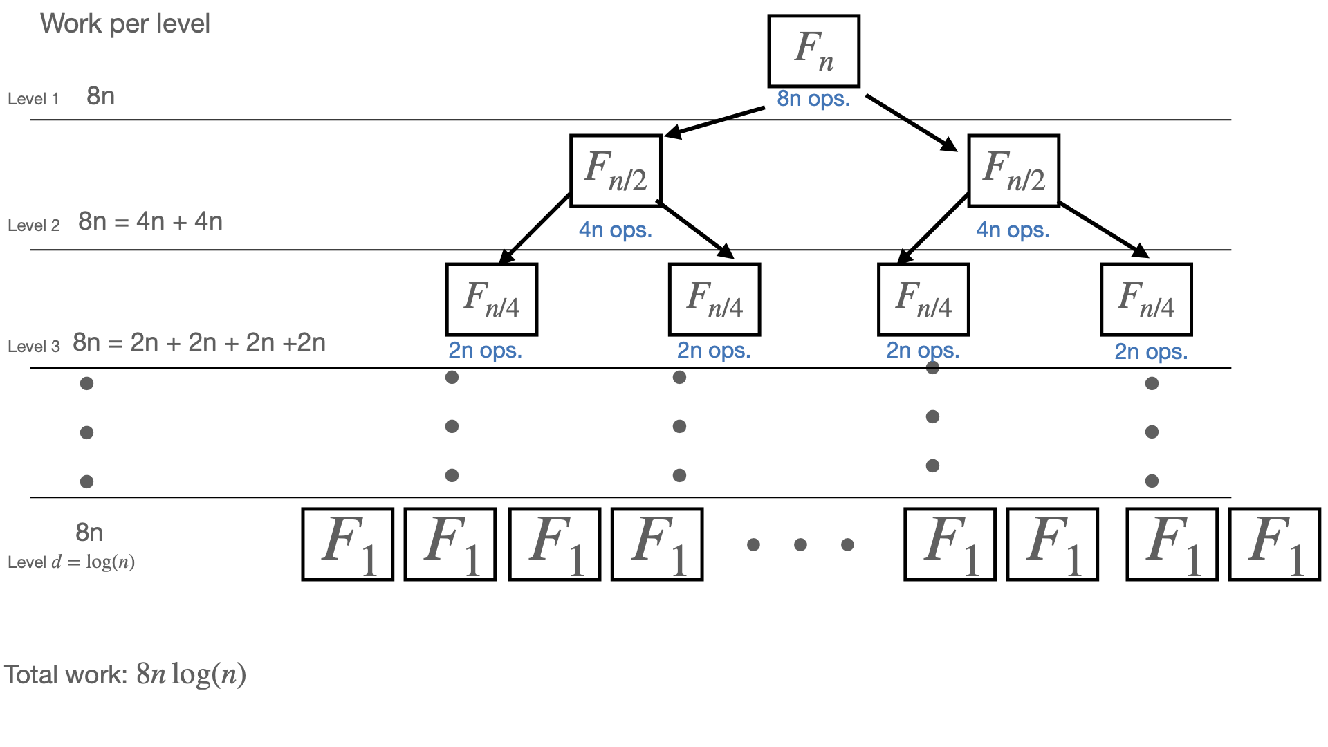
At the top of the tree, we seek a DFT of size $n$ which we "divide-and-conquer" into two DFTs of size $n/2$, we then scale and add those vectors which takes $8n$ operations. At next level, where we compute two $F_{n/2}$, we do $8(n/2)$ work to scale/add vectors, thus $8 (n/2) \times 2 = 8n$ total work. Recursively, we see that we do $8n$ work at each level of the tree. After $\log_2(n) = d$ rounds of divide and conquer, we hit the base case of $n =1$, for which $F_1x = x$. Summing up the work of each level, we thus do $ ~ 8n d = 8n \log_2 n$ work.

Figure: Illustration of computational complexity of the FFT

Write a recursive algorithm for the DFT assuming $n = 2^d$.

import numpy as np
def my_fft(x): 
    n = x.size
    ## ADD YOUR CODE HERE
    return x*0

## Code below is provided for you. No need to change it.
n=2**10
x = np.random.randn(n) + np.random.randn(n) * 1j
y = np.fft.fft(x)
# Should be close to machine epsilon. ~1e14 is fine
print("error: ",np.linalg.norm(y - my_fft(x)) / np.linalg.norm(y))

Q2. Chebyshev polynomials

The Chebyshev polynomials are defined from the three-term recurrence relation:

$$T_0(x) =1, \quad T_1(x) = x, \quad T_{n+1}(x) = 2xT_n(x) - T_{n-1}(x) $$

The Chebyshev polynomials are the numerical analyst's favorite polynomials because of all of their wonderful properties. For example, we showed in class they have astonishing closed form: $T_n(x)= \cos(n\arccos(x))$. Using this property, it is straight-forward to see that the roots of the Chebyshev polynomial $T_n(x)$ are:

$$ x_i = \cos \left( \frac{2i -1 }{2n}\pi \right), \quad i = 1, \dots n $$

These points are known as the Chebyshev nodes (of the first kind).

2.1 Clenshaw's algorithm

Using the three-term recurence, implement an algorithm to evaluate the sum $p_n(x) = \sum_{k=0}^{n} c_k T_k(x) $ in $\mathcal{O}(n)$ operations. This method is called Clenshaw's algorithm and is applicable to any polynomials with a three-term recurrence.

import numpy as np 

def clenshaw(c, x):
    # Computes \sum_{i=0}_{n} c_i T_i(x)
    # where c is a (n+1) sized vector and T_i(x) is the i-th Chebyshev polynomial
    # x is a scalar
    n = c.size - 1
    sum =0
    ## ADD YOUR CODE HERE
    return sum

## Code below is provided for you. No need to change it.

# Test
c = np.random.randn(10)
x = 0.1
# Compare to built in method. Should be close to machine epsilon ~1e-15
print('error :', np.abs(np.polynomial.chebyshev.chebval(x, c) - clenshaw(c, x)))

Q2.2: Interpolant

Write a function that computes the chebyshev expansion of the Chebyshev interpolant of a function $f(x)$. That is, given an input vector $b\in \mathbb{R}^{n+1}$ with $b_i = f(x_i)$ where $x_i = \cos(\frac{2i -1 }{2(n+1)}\pi)$ for $i = 1, \dots (n+1)$ , compute the output vector $c \in \mathbb{R}^{n+1} $ so that the polynomial $p_n(x) = \sum_{i=0}^n c_i T_i(x) $ satisfies $p_n(x_i) = f(x_i)$.

Write this problem as the solution of a linear system, similar to the Vandermonde matrix approach discussed in class. Use the three term recurrence to fill the entries of the matrix (not the cosine formula!).

(Optional) This implementation is $\mathcal{O}(n^3)$, but there is an $\mathcal{O}(n \log n)$ algorithm to perform this computation using the FFT through the Discrete Cosine Transform (DCT), you can read about it here https://en.wikipedia.org/wiki/Discrete_Chebyshev_transform and implement it using scipy.fftpack.dct.

def fit_chebyshev_pol(f):
    # f is a vector of size (n+1)
    # returns the (n+1) coefficients of the n degree interpolant in the chebyshev basis 
    n = f.size-1

    ## ADD YOUR CODE HERE

    return f*0

## Code below is provided for you. No need to change it.

# A Helper function to get n roots of the T_n(x)
def get_cheb_nodes(n):
    return np.cos((2 * np.arange(1, n+1) - 1)/( 2* n) * np.pi )

n = 10
f_fn = lambda x : np.cos(3*np.pi*x) * np.exp(x)
x = get_cheb_nodes(n)
f = f_fn(x)
c = fit_chebyshev_pol(f)

# Evaluate the interpolant. Should get the values back! Up to ~ 1e-14 is fine
print(np.linalg.norm(np.polynomial.chebyshev.chebval(x, c) - f) )

Q2.3. Clenshaw-Curtis quadrature

In class, we defined the Newton-cotes quadrature as the integral of the equispaced interpolant. Similarly, Clenshaw-curtis quadrature is the integral of the Chebyshev interpolant.

$$ \int_{-1}^1 f(x) dx \approx \int_{-1}^1 p_n(x) dx = \sum_{i=0}^n w_i f(x_i) $$

Using a similar idea as 2, and the following identity:

$$ \int_{-1}^1 T_n(x)\, \mathrm{d}x = \begin{cases} \frac{(-1)^n + 1}{1 - n^2} & \text{ if }~ n \ne 1 \\ 0 & \text{ if }~ n = 1. \end{cases} $$

write a function that computes the Quadrature weights. That is, find a vector $w\in \mathbb{R}^{n+1}$ so that

$$ \int_{-1}^1 p_n(x) dx = \sum_{i=0}^n w_i f(x_i) = w^T b $$

where $x_i$ are the Chebyshev nodes of degree $(n+1)$. Note that these weights, like the Newton-Cotes weights, do not depend on the function $f$.

Optional: compute the weights in $\mathcal{O}(n \log n) $.

def get_Clenshaw_Curtis_weights(n):
    # returns a vector of (n+1) weights of the n-th order Clenshaw-curtis quadrature:

    # ADD YOUR CODE HERE

    return np.zeros(n+1)

## Code below is provided for you. No need to change it.

n = 4
w = get_Clenshaw_Curtis_weights(n)
cc_w = np.array([0.16778123, 0.5255521 , 0.61333333, 0.5255521 , 0.16778123])
print('error (should be ~1e-8):', np.linalg.norm( w - cc_w))

Q2.4. Spectral convergence of Clenshaw-curtis

Use your quadrature rule to estimate the integral of the smooth function:

$$ \int_{-1}^1 \cos(3 \pi x) \exp(x) dx $$

Make a plot displaying the spectral convergence of the method. The analytical value of the integral is given below so that you may compute the error.

import matplotlib.pyplot as plt
f_fn = lambda x : np.cos(3*np.pi*x) * np.exp(x)

# The analytical value of the integral 
analytical_integral = (1 - np.exp(2) )/( np.exp(1) + 9 * np.exp(1) * np.pi**2)

nns = np.arange(1,50)
errors = np.zeros(nns.size)
for n_idx,n in enumerate(nns):
    # ADD YOUR CODE HERE
    errors[n_idx] 

plt.semilogy(nns,errors)

Q3. Solving PDEs: beyond Poisson's equation

In this exercise, we approximate solutions to elliptic PDEs of the form:

$$ - \frac{d^2}{dx^2} u(x,y) - \frac{d^2}{dy^2}u(x,y) + c(x,y)u(x,y) = f(x,y)\\ \qquad u(x,0) = u(x,1) =0\\ \qquad u(0,y) = u(1,y) = 0 $$

where $c(x,y) \geq 0$. Last HW, we solved Poisson's equation on the square with homogeneous Dirichlet conditions:

$$ - \frac{d^2}{dx^2} u(x,y) - \frac{d^2}{dy^2}u(x,y) = f(x,y)\\ \qquad u(x,0) = u(x,1) =0\\ \qquad u(0,y) = u(1,y) = 0 $$

This is equivalent to the above equation with $c(x,y) = 0$. We saw that using finite differences, the Poisson PDE may be discretized as:

$$ TU + UT = F $$

where $T$ is the tridiagonal second-order finite difference matrix, and $F_{i,j} = h^2 f(x_i, y_j)$ with $x_i = i h $, $y_j = jh$, and $h = \frac{1}{n+1}$. To discretize the modified equation, we only need to account for the additional operator $u \to c u$. Since both $c(x,y)$ and $u(x,y)$ are discretized on a grid and $(cu)(x_i, y_j) = c(x_i, y_j)u(x_i, y_j)$, this operator is represented as:

$$ C \cdot U $$

where $\cdot$ is a pointwise multiplication between the two matrices (also called the Hadamard product), and C is the matrix $C_{i,j} = h^2 c(x_i, y_j)$.

Thus, the discretized system becomes:

$$ TU + UT + C\cdot U = F $$

In the previous homework, we solved Poisson's equation in only $\mathcal{O}(n^2 \log n)$ time by recognizing it as a Sylvester equation and using the Bartels-Stewart algorithm, leveraging the diagonalization of $T$. However, this new equation is not a Sylvester equation, so those methods no longer apply.

We turn instead to the Kronecker product formalism introduced in Homework 3. The pointwise multiplication $C \cdot U$ can be equivalently expressed in vectorized form as $\text{vec}(C) \cdot \text{vec}(U)$, or equivalently as $D \text{vec}(U)$, where $D = \text{diag}(\text{vec}(C))$ is the diagonal matrix of size $\mathbb{R}^{n^2 \times n^2}$ with $\text{vec}(C)$ on its diagonal.

This reformulation gives:

$$ TU + UT + C \cdot U = F \Leftrightarrow \left( (I \otimes T) + (T \otimes I ) + D \right) \text{vec}(U) = \text{vec}(F) $$

One way to solve this system is by explicitly forming the matrix $A = \left((I \otimes T) + (T \otimes I) + D\right)$ and performing a dense linear solve. However, this approach requires $\mathcal{O}(n^6)$ operations, which is computationally prohibitive. Instead, we leverage fast matrix-vector products with $A$, making this system ideal for Krylov subspace methods. Since $T$ is symmetric positive definite (SPD), $A$ is also SPD, allowing us to use the conjugate gradient (CG) method.

Q3.1

Implement a function that computes the matrix-vector product with a vectorized version of $Ax$ in $\mathcal{O(n^2)}$ operations. Note that A is of size $n^2 \times n^2$, so this is a linear-time matvec in the size of a vector. Then, using the built-in CG iteration, run CG for 20 iterations, asking to stop if tolerance tol drops below $10^{-8}$. You can run CG using the following command xk,info = scipy.sparse.linalg.cg(A_op, b, maxiter=maxiter, tol = tol, callback=callback), the callback functions will allow you to store the residual at each step (which CG does not do by default).

Note that we take $n = 1000$, so A has one million rows and columns: no way we could do a dense solve (a back of the envelope calculation estimates it would take two years of compute time!).

import scipy
import scipy.sparse
import matplotlib.pyplot as plt
import scipy.sparse.linalg
import numpy as np

def diff_eq_mat_vec(C, x):
    # Implement the Ax in O(n^2) where x in an n^2 vector and 
    # A is the matricized version of the operator
    # X -> TX + XT + C dot X

    # ADD YOUR CODE HERE

    return 0*x

# Helper functions for you to use - READ THEM!

# returns the T matrix in sparse format.
# T@x where x is a vector is an O(nnz) operations where nnz is the number of non zeros in T 
# Since T has ~3n non zeros, T@x is an O(n) operation 
def get_sparse_T(n):
    T = scipy.sparse.diags([np.ones(n-1), -2*np.ones(n), np.ones(n-1) ], offsets = [-1, 0, 1])
    return T

# Vectorization of matrix
def vec(X):
    return X.T.reshape(-1)

## Inverse of vec function.
def unvec(x):
    n = np.sqrt(x.size).astype(int)
    return x.reshape(n,n).T


### A test for the MATVEC.
n = 10
C = np.linspace(1.2, 1.5, n**2).reshape(n,n)
T = get_sparse_T(n).A
I = np.eye(n)
# Write down the big kron matrix
A = np.kron(I, T) + np.kron(T, I) + np.diag(vec(C))

x = np.linspace(1, 4, n**2)
y = diff_eq_mat_vec(C,x)
print('error in mat_vec (n=10): (should be ~1e-14)', np.linalg.norm(y-A@x))

We define the coefficients below. Use your fast-matvec to attempt solving the linear system by calling CG below. What do you observe about the convergence of CG? How big is the residual after 20 iterations?

# Defining the coefficients of a PDE
c_fun = lambda x,y : np.sin(3*np.pi * x  * y)**2 * y
f_fun = lambda x,y : np.exp( -( x**2 +  y**2)) * ( np.cos(10*np.pi * y)  +  np.sin(4*x)**2)

# Discretization size
n = 1000 # If your computer struggles with n = 300, if not, try n =3000!

# Generate the grid
xgrid = np.linspace(0, 1, n)
xx, yy = np.meshgrid(xgrid, xgrid)
#Evaluate c_fun and f_fun on grid.
C = c_fun(xx,yy) * (1/(n+1)**2)
F =  f_fun(xx,yy) * (1/(n+1)**2)
b = vec(F)

# To run CG, we need to pass to scipy a blackbox A_mv(x) that implements A @ x fast
# Below the required syntax. You can look up the documentation,
# but it isn't important, nothing very interesting is happening
A_matvec = lambda x : diff_eq_mat_vec(C, x)
# Wraps the matvec into a format expected by scipy
A_op = scipy.sparse.linalg.LinearOperator((n**2,n**2), A_matvec)

# To record residuals at each iteration, we need to give this callback function as an input
residuals = []
# Define callback function to store residual at each iteration
def callback(xk):
    residual = np.linalg.norm(A_op @ xk - b) / np.linalg.norm(b)
    residuals.append(residual)


### ADD YOUR CODE HERE !!! CALL CG
## add callback=callback as an argument to compute and store the residual at each iteration
xk,info = scipy.sparse.linalg.cg(callback = callback)

plt.plot(residuals, marker='o')
plt.yscale('log')  # Log scale for better visualization of convergence
plt.xlabel('Iteration')
plt.ylabel('Relative Residual')
plt.title('Convergence of CG Solver')
plt.grid(True)
plt.show()

# Plots approximate solution
plt.imshow(unvec(xk))
plt.title('computed approximate solution of PDE')
plt.colorbar()

The slow convergence behavior above is typical when solving linear systems obtained by discretizing differential equations. Recall the CG convergence bounds that

$$ \frac{\|e_k\|_A}{\|e_0\|_A} \leq 2 \left( \frac{ \sqrt{\kappa(\mathbf{A})}-1 }{ \sqrt{\kappa(\mathbf{A})}+1 } \right)^k \approx 2 \left( 1 - \frac{2}{\sqrt{\kappa(\mathbf{A})}} \right)^k \, $$

where $K_2(A)$ is the condition number of A, thus when $K_2(A)$ is large, the convergence may be very slow. Also recall that when A is SPD: $$K_2(A) = \|A\|_2 \|A^{-1}\|_2 = \frac{ \sigma_{max}(A)}{\sigma_{min}(A)} = \frac{ \lambda_{max}(A)}{\lambda_{min}(A)} $$

The discretization by finite difference of second-order differential operator (such as the ones here) have condition number that grows proportionally to $n^2$: $K_2(A) = \mathcal{O}(n^2)$ so we expect very poor convergence for even moderately large $n$.

We are missing one last ingredient in our PDE solver: a preconditioner. Preconditioning is the idea of replacing a linear system $Ax=b$ with a different, but equivalent linear system $M^{-1}Ax = M^{-1}b$. The matrix $M$ is called the preconditioner. A good preconditioner should have two properties:

• $K_2(M^{-1}A)<< K_2(A)$, so the iterative method applied to this new system converges fast.
• $M^{-1}$ is easy to compute so that each iteration is fast.

Running preconditioned CG on the matrix $A$ with preconditioner $M$ is mathematically equivalent to running the original CG on $L^{-1}A(L^{-1})^T$ where $LL^T = M$, so to bound the condition number of $L^{-1}A(L^{-1})^T$, it is sufficient to bound the eigenvalues of $M^{-1}A$ or $L^{-1}A(L^{-1})^T$ as these are similar matrices. See notes for lecture 18 if this is unclear!

Preconditioners are highly problem specific. They are often the special sauce that, together with a Krylov method, makes a modern numerical method blazingly fast. As such, they are the basis for much research interest. Often, the trick to finding a good preconditioner is to find a "nearby" but easier problem. In our case, we can pick $M$ to be the discretization of Poisson's equation: $M = T \otimes I + I \otimes T$. In this case, we have that $A = M + D$, where $D=\text{diag}(\text{vec}(C))$, and one can show that $L^{-1}A(L^{-1})^T$ is well conditioned.

Q3.2

Proving that the preconditioned system is well conditioned is your next ask. Since we know the exact eigenvalue decomposition of $T$ (see previous HW) it is easy to bound eigenvalues of $M = T \otimes I + I \otimes T$.

$$ \lambda_{\text{min}}(M) \approx \frac{2 \pi^2}{(n+1)^2}, \quad \lambda_{\text{max}}(M) = 8 $$

Using these estimates show that $L^{-1}A(L^{-1})^T$ is well conditioned, specifically, show that:

$$ K_2( L^{-1}A(L^{-1})^T ) \leq 1 + \frac{1}{2\pi^2}\max_{x,y}{c(x,y)} \ .$$

(You may use the $\approx$ in $\lambda_{\text{min}}(M)$ as equality). Note that the bound is independent of $n$ and small if $c(x,y)$ doesn't get too large, so we expect CG to converge very quickly. In our case, $c(x,y) \leq 1 $ so we expect very fast convergence.

Hint: You can (but do not have to) use the following characterization of the eigenvalues of symmetric matrices based on the Rayleigh quotient:

$$ \lambda_{max}(B) = \max_{x \in \mathbb{R}^n} \frac{x^TBx}{x^Tx} \ , \\ \lambda_{min}(B) = \min_{x \in \mathbb{R}^n} \frac{x^TBx}{x^Tx} \ , $$

also recall that $c(x,y) \geq 0$, $C_{i,j} = h^2 c(x_i,y_j) $.

Q3.2 ADD YOUR ANSWER HERE

Q3.3

Implement your preconditioner in my_poisson_preconditioner (based on HW4). Then pass it as an input to CG using the M option: scipy.sparse.linalg.cg(A_op, b, M= M_op, maxiter =20, tol = 1e-8, callback=callback ) . Compute the residual once more. What do you observe?

def my_poisson_preconditioner(b):
    ## Should compute M^{-1} b

    ## ADD YOUR CODE HERE. NOTE YOU SHOULD ALSO ADD YOUR CODE BELOW!
    return b*0

# A helper function you can use if you want
def dst(X,axis =0):
    return scipy.fft.dst(X, type = 1, norm = "ortho", axis =axis)

# Computes eigenvalues of the Tridiagonal matrix from known analytical formula
def get_eigenvalues_of_T(n):
    return 4 * (np.sin(np.arange(1,n+1) * np.pi / (2*( n + 1)))**2)

# Wraps M_op(x) =  M^{-1} @ x in a format scipy expects
M_op = scipy.sparse.linalg.LinearOperator((n**2,n**2), my_poisson_preconditioner)

# To record residuals at each iteration
residuals = []
# Define callback function to store residual at each iteration
def callback(xk):
    residual = np.linalg.norm(A_op @ xk - b) / np.linalg.norm(b)
    residuals.append(residual)

## ADD YOUR CODE HERE!!
## ADD YOUR CODE HERE!!
## ADD YOUR CODE HERE!!

# Call CG to solve the system A * x = b with callback
## add callback=callback as an argument to compute the residual at each iteration
xk,info = scipy.sparse.linalg.cg(callback=callback)
plt.figure()
# Should converge very fast ! only 4-5 iterations and we are done
# Plot convergence of the residual
plt.plot(residuals, marker='o')
plt.yscale('log')  # Log scale for better visualization of convergence
plt.xlabel('Iteration')
plt.ylabel('Relative Residual')
plt.title('Convergence of CG Solver')
plt.grid(True)
plt.show()

Much better convergence! Note that our first approximate solution looks visually nothing like our correct one.

There is a lot more to be said about numerical solvers for PDEs such as handling more complicated domains, handling coupled PDEs and dealing with nonlinearities, but we have now seen the entire lifespan of a typical linear PDE solver:

• A discretization scheme is used to turn a continuous problem into a linear system.
• An iterative method is chosen, often CG or GMRES, to solve the linear system.
• A preconditioner is devised to speed up convergence.

Q4 Alternating direction implicit

In class, we proved the convergence of Krylov subspace methods through a connection with a polynomial approximation problem. This link between numerical linear algebra and approximation theory is pervasive, and we see another example here with a different iterative solver: the Alternating Direction Implicit (ADI) method. ADI is an iterative solver for Sylvester equations:

$$ AX - XB = F $$

It is defined as the following iteration:

$X^{(0)} = 0$

for $j=0,1,2,3,\dots$

Solve for $X^{(j + 1/2)}$, where $\left( A - \beta_{j +1} I\right) X^{(j+1/2)} = X^{(j)}\left( B - \beta_{j + 1} I \right) + F$

Solve for $ X^{(j + 1)}$, where $ X^{(j+1)}\left( B - \alpha_{j + 1} I \right) = \left( A - \alpha_{j+1} I\right) X^{(j+1/2)} - F$

The scalars $\alpha_j$ and $\beta_j$ are hyperparameters that must be chosen a priori.

1. Show the following identity:

$${\displaystyle X-X^{(K)}=\left(\prod _{j=1}^{K}{ {(A-\alpha _{j}I)(A-\beta _{j}I)^{-1}} } \right) \left(X-X^{(0)}\right) \left( \prod _{j=1}^{K}{ {(B-\beta _{j}I)(B-\alpha _{j}I)^{-1} }} \right) }$$

where $X$ is the solution to the Sylvester equation.

Hint: Note that $F = AX - XB + (- \beta_{j+1} X + \beta_{j+1} X) = (A - \beta_{j +1} I)X - X\left( B - \beta_{j + 1} I \right) $.

Let $E^{(j)} = X - X^{(j)}$. First show that

$$E^{(j + 1/2)} = \left( A - \beta_{j +1} I\right)^{-1} E^{(j)}\left( B - \beta_{j + 1} I \right) \ , $$

then derive a similar relation between $E^{(j + 1)}$ and $E^{(j + 1/2)}$ and combine them to show the identity.

Use 1 to show:

$$ \frac{\| \displaystyle X-X^{(K)}\|_2}{ \|X\|_2 } \leq \|r_K(A)\|_2 \| r_K(B)^{-1}\|_2 $$

where $r_K(x)$ is the rational function: $$r_K(x) = \prod_{j=1}^K \frac{x - \alpha _{j}}{x - \beta _{j}} \ . $$ The function applied to the matrix is defined as: $r_K(M) = \prod_{j=1}^{K}{ {(M-\alpha _{j}I)(M-\beta _{j}I)^{-1}} }$.

Hint: you may use the fact that all matrices of the form $(M - \alpha I)$ for any $\alpha \in \mathbb{C}$ (and their inverses) commute with each other, for example: $(M-\alpha I)(M-\beta I)^{-1} =(M-\beta I)^{-1}(M-\alpha I)$ (you should convince yourself this is true!).

Assume that $A$ and $-B$ are SPD. Show that:

$$ \frac{\| \displaystyle X-X^{(K)}\|_2}{ \|X\|_2 } \leq \frac{ \sup_{\lambda \in [ a ,b ]} |r_K(\lambda )|}{ \inf_{\lambda \in [ -d, -c]} |r_K(\lambda )| } $$

where $a = \lambda_{\text{min}}(A) $, $b = \lambda_{\text{max}}(A) $, $c = \lambda_{\text{min}}(-B) $, $d = \lambda_{\text{max}}(-B) $

Thus, one should pick the shifts $ \alpha_j$ and $\beta_j$ such that the right-hand side is as small as possible. In other words, $r_K(x)$ must solve the following rational function approximation problem:

$$ \gamma(K, a, b,c,d) = \inf_{\lambda_j, \alpha_j} \frac{ \sup_{\lambda \in [ a ,b ]} |r_K(\lambda )|}{ \inf_{\lambda \in [ -d, -c]} |r_K(\lambda )| } $$

The approximation problem is known as Zolotarev's third problem. A solution is known in the case that $a = d$, and $c = b$, which corresponds to the case when $B = -A$. The optimal $\alpha_j,\beta_j$ are not easy to write down, but for our purposes, it is sufficient to know they exist, and that

$$\gamma(K, a, b,a,b) =4 \left[\exp\left( \frac{\pi^2}{2 \log (4b/a)} \right) \right]^{-2K} \ .$$

Use this result to prove that the error in ADI satisfies $\|E^{(K)}\| = \mathcal{O}(\rho^K)$ for some $\rho <1$ (that is, it converges at least linearly in $K$) when $B = -A$, $A$ is SPD, and the optimal shifts are used.

ADD YOUR ANSWER TO QUESTION 4 HERE

Q5: Gauss-Legendre Quadrature

In class, we showed that, given a fixed set of distinct quadrature nodes $\{x_k\}_{k=1}^n$, we can always find quadrature weights so that the quadrature rule integrates all polynomials of degree $n-1$ exactly, that is:

$$ \int_a^b p(x)\,dx = \sum_{k=1}^n w_k p(x_k) $$

for all polynomials $p(x)$ of degree at most $n-1$.

In this question, we show that by choosing the nodes $\{x_k\}_{k=1}^{n}$ as the roots of the $n$-th Legendre polynomial $P_n(x)$ (with weights chosen as above), we can integrate polynomials of degree $2n-1$. This is called Gauss-Legendre quadrature and is the default choice for integrating smooth functions.

The key step uses polynomial division (see polynomial long division if needed). For any polynomial $p(x)$ with $\deg p \le 2n-1$, the decomposition $$ p(x) = q(x)P_n(x) + r(x) $$ with $\deg q \le n-1$ and $\deg r \le n-1$ always exists and is unique.

5.1

Show that $\int_{-1}^{1} q(x)P_n(x)\,dx = 0$.

5.2

Let $x_1, \ldots, x_n$ be the roots of $P_n(x)$ (the Gauss-Legendre nodes), and let $Q_n(f) = \sum_{k=1}^n w_k f(x_k)$ be the Gauss-Legendre quadrature rule.

Show that $Q_n(p) = Q_n(r)$.

5.3

Using Steps 1 and 2, and assuming the weights are chosen so that the quadrature rule is exact for polynomials of degree at most $n-1$, show that $$ Q_n(p) = \int_{-1}^1 p(x)\,dx $$ for all polynomials $p(x)$ of degree at most $2n-1$. This shows that Gauss-Legendre quadrature with $n$ nodes is exact for all polynomials of degree up to $2n-1$ (which is optimal).

ADD YOUR ANSWER TO QUESTION 5 HERE

Extra credit:

• Solvers based on ADI this paper, this paper
• Non-uniform fast Fourier transform this paper, this one
• Using orthogonal polynomials this paper, this paper