Quick Start
What you'll need
| Requirement | Details |
|---|---|
| Particle stack | A .star file (RELION) or .cs file (cryoSPARC) with CTF parameters |
| Mask | A .mrc binary mask covering your molecule of interest |
| GPU | An NVIDIA GPU (Volta or newer). 16+ GB VRAM is recommended; less works for smaller boxes or with --downsample / --lazy (40+ GB helps for large datasets at 256px) |
| RECOVAR installed | pip install "recovar[gpu]" for pipeline use; add pip install "recovar[gui]" for GUI support. See Installation for details |
Timing
A small dataset (~50k particles at 128px) takes about 10 minutes end-to-end. Larger datasets (500k+ particles at 256px) may take 30--60 minutes.
Run your first job
Key terms
- zdim: Number of latent-space dimensions. A first run with
zdim=4is a good default (it's what the GUI uses); increase to 10 or 20 to resolve finer heterogeneity at the cost of speed. - K-means: Groups particles into representative conformational states.
- UMAP: 2D visualization of the latent space for exploring heterogeneity.
- Eigenvolumes: Volume representations of the principal components; the ones that look like noise can be dropped when choosing zdim.
- Trajectory: A series of volumes showing a conformational path between two states.
1. Launch the GUI
This opens a browser window at http://localhost:8080.
2. Create a project and submit a pipeline job
- Click Create Project and choose a directory
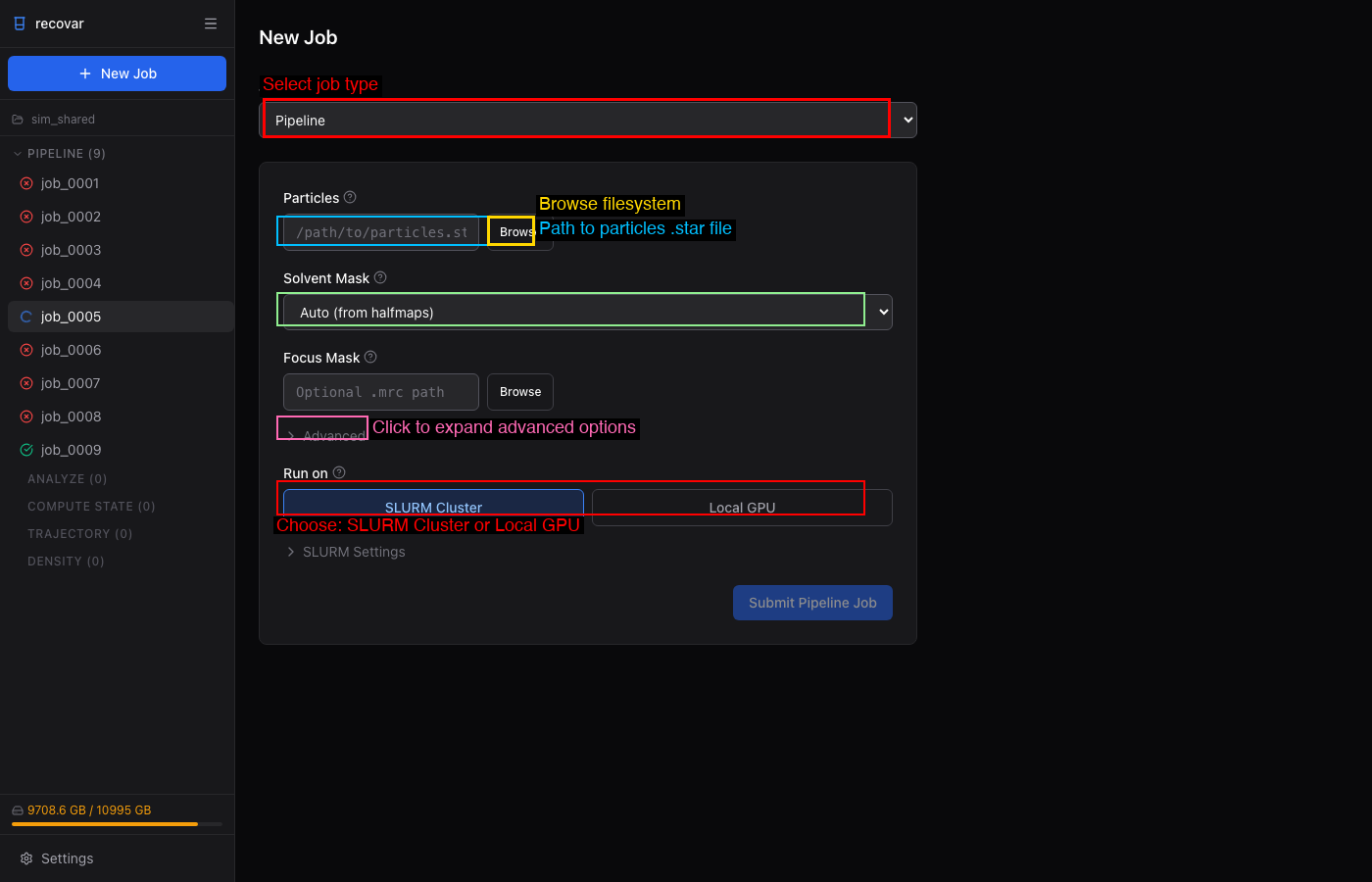
- Click New Job > Pipeline
- Browse to your particles file (
.staror.cs) - Select a mask (or use Auto/Sphere)
- Click Submit Pipeline Job
3. Analyze results
Once the pipeline completes, click Analyze this pipeline output in Next Steps. The zdim defaults to 4 (good for a first look — raise it to 10 or 20 for finer detail), then click Submit Analyze Job.
4. Explore
The GUI shows eigenvalue spectra, UMAP scatter plots, and lets you click to generate volumes at any point in latent space. See the GUI Guide for details.
1. Interactive wizard (recommended for first-time users)
The wizard walks you through selecting input files, mask, downsampling, and other options, then runs the pipeline. Works over SSH.
2. Or run directly
recovar init_project my_project
cd my_project

# RELION
recovar pipeline particles.star --mask mask.mrc --project .

# cryoSPARC
recovar pipeline particles.cs --mask mask.mrc --datadir /path/to/cryosparc/project --project .

# Analyze
recovar analyze --zdim=10 --project .
3. View volumes
Open .mrc files in ChimeraX or any MRC viewer:
If you prefer explicit output directories (no project system):
Expected output after each step
After recovar init_project: Creates the project directory with a project.json index file.
After recovar pipeline: Creates Pipeline/job_0001/ containing:
output/volumes/mean.mrc,mean_half1_unfil.mrc,mean_half2_unfil.mrc-- mean reconstruction and half-mapsoutput/volumes/eigen_pos0000.mrc, ... andvariance*.mrc-- eigenvolumes and variance mapsoutput/plots/-- diagnostic plots (eigenvalue spectrum, etc.)model/-- internal results:params.pkl,embeddings.pkl, and per-zdim coordinates undermodel/zdim_<N>/job.json,command.txt,run.log-- run metadata
After recovar analyze: Creates Analyze/job_0001/ (or analysis_<zdim>/ when run with -o) containing:
kmeans/center000.mrc,center001.mrc, ... -- cluster center volumesdata/kmeans_result.pkl-- k-means labels and centersplots/PCA/,plots/umap/-- PC scatter and UMAP plots
With downsampling
If your images are larger than ~256 pixels, downsample for faster processing:
This pre-downsamples images into the shared project cache on the first run and reuses that cache across matching project runs.
Project system
The project system is the standard RECOVAR workflow. Numbered job directories stay stable on disk (e.g. Pipeline/job_0001/, Analyze/job_0001/), while the CLI and GUI show human-readable job names from project metadata.
recovar init_project my_project
cd my_project
recovar pipeline particles.star --mask mask.mrc --project .
recovar analyze --zdim=10 --project .
recovar project_status
All commands accept --project <dir> to enable project mode. If you run from within a project directory, it is auto-detected.
Next steps
- Web GUI -- launch the browser interface to interactively explore latent spaces and view 3D volumes
- Analyzing Results -- deep dive into k-means, trajectories, UMAP, and volume generation options
- Input Data -- supported formats and data preparation
- Downsampling -- when and how to downsample