Analyzing Results

After the pipeline finishes, use recovar analyze to generate volumes, compute k-means clusters, create trajectories, and run UMAP.

Choose your workflow: CLI or GUI

This page has tabbed instructions for both the command line and the web GUI. Click the tab headers below each section to switch. Your choice is remembered across all pages. How to launch the GUI →

Submitting an analyze job

GUI CLI

1. From a completed pipeline job, click Analyze this pipeline output in Suggested Next Steps (auto-fills the result directory)
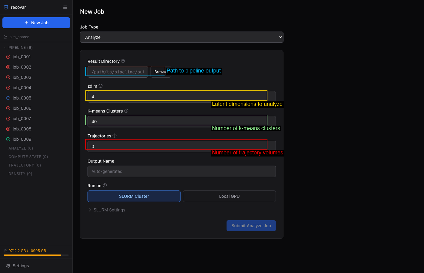
2. Or click + New Job > Analyze and browse to the pipeline output directory
3. Set zdim, k-means clusters, and trajectories
4. Optionally expand Advanced to tune n-bins and maskrad-fraction (the kernel-regression knobs that trade resolution for speed)
5. Click Submit Analyze Job

Quick Analyze

The Quick Analyze button submits the same job with n-bins=10 and maskrad-fraction=10, which makes the cluster-center volumes roughly 40x faster to compute at a lower resolution. UMAP and k-means clustering are unchanged. It's a good way to preview the conformational landscape before running a full-resolution analysis.

recovar analyze output --zdim=10

This generates:

• K-means cluster centers and their volumes
• UMAP embedding of the latent space
• Trajectories between cluster pairs (if requested)

Results are saved next to the pipeline output, in result_dir/analysis_10/ (here result_dir is output). With --no-z-regularization, the suffix changes and results go to result_dir/analysis_10_noreg/.

Options

Flag	Default	Description
--zdim	Auto	Latent dimension (single integer). If the pipeline produced only one embedding, it is used automatically; otherwise you must set this
-o	Auto	Output directory (default: result_dir/analysis_{zdim}/, or analysis_{zdim}_noreg/ with --no-z-regularization)
--n-clusters	20	Number of k-means clusters
--n-trajectories	0	Number of trajectories between cluster pairs
--n-vols-along-path	6	Volumes per trajectory
--Bfactor	0	B-factor sharpening
--n-bins	50	Bins for kernel regression
--maskrad-fraction	20	Kernel radius = grid_size / maskrad-fraction. Lower it for noisier data, raise it for low-resolution data
--n-min-particles	100	Minimum particles per bin for kernel regression
--skip-umap	False	Skip UMAP (faster for large datasets)
--skip-centers	False	Skip generating cluster center volumes
--lazy	False	Lazy loading for large datasets
--no-z-regularization	False	Use unregularized latent variables (changes output suffix to _noreg)

How to choose zdim

Look at the eigenvalue spectrum plot. Choose the zdim where eigenvalues start to flatten -- this is where signal transitions to noise. Typical values: 2-4 for simple motions, 10-20 for complex heterogeneity.

What to inspect first after analyze

1. Mean map — is the reconstruction sensible? Open mean_filt.mrc in ChimeraX
2. Eigenvalue spectrum — how many modes before it flattens? That's your signal
3. PCA scatter — isolated clusters or continuous gradients?
4. K-means volumes — do the differences correspond to real density changes?
5. UMAP — does it confirm the structure seen in PCA?
6. Subsets — export only after visually inspecting volumes, not just scatter plots

Sampling many states

To sample many conformational states (e.g., 100-200), use --n-clusters=200 and --n-bins=10 for speed, then recompute selected states at higher resolution with compute_state.

Generating volumes at specific points

Use compute_state to generate volumes at specific coordinates in latent space:

recovar compute_state output -o volumes \
    --latent-points coords.txt --Bfactor=50

The coordinates file is a text file with shape (n_points, zdim), readable by np.loadtxt. You can use the k-means centers from analyze:

recovar compute_state output -o volumes \
    --latent-points output/analysis_10/kmeans/centers.txt --Bfactor=50

Options

Flag	Default	Description
--latent-points	Required	Coordinates file (.txt)
--Bfactor	0	B-factor sharpening
--n-bins	50	Bins for kernel regression
--maskrad-fraction	20	Kernel radius = grid_size / maskrad_fraction
--n-min-particles	100	Minimum particles for kernel regression
--particles	Same	Different particle stack for higher resolution
--datadir	Same	Path prefix for particle paths

Computing trajectories

Use compute_trajectory to compute high-density paths through latent space:

recovar compute_trajectory output -o trajectory --zdim=10 \
    --density density/data/deconv_density_knee.pkl \
    --endpts centers.txt --ind 0,1

Specifying endpoints

Choose one of:

Method	Flags	Description
From coordinate file	--endpts file.txt --ind 0,1	Lines 0 and 1 of the file
Separate files	--z_st start.txt --z_end end.txt	One coordinate per file
From coordinate file	--endpts file.txt	Uses first two lines

Options

Flag	Default	Description
--zdim	Auto	Latent dimension. Inferred from the embedding when only one is present; set it when several are available
--density	None	Density file for high-density path
--n-vols-along-path	6	Number of volumes along the path
--Bfactor	0	B-factor sharpening
--n-bins	50	Bins for kernel regression

Tip

The --density option is important for computing paths that follow high-density regions. Generate density with estimate_conformational_density.

Viewing results

Interactive exploration

Use recovar gui to explore results interactively in your browser — view scatter plots, click to generate volumes, and inspect 3D renderings. See the GUI Guide.

Volume files

Open .mrc files in ChimeraX, Chimera, or any MRC viewer:

output/analysis_10/
  kmeans/
    center000.mrc              # K-means center 0
    center001.mrc              # K-means center 1
    center000_half1_unfil.mrc  # Half-map 1 (for FSC)
    ...
    centers.txt                # Center coordinates
    diagnostics/center000/     # Per-volume diagnostics
  traj000/
    state000.mrc               # Start of trajectory
    state001.mrc               # Along trajectory
    ...
    diagnostics/state000/      # Per-volume diagnostics

UMAP plots

UMAP embeddings are saved in the analysis directory. Use the Jupyter notebook kernel (recovar) for interactive visualization.

Trajectory movies

Load the trajectory volumes as a series in ChimeraX to create conformational movies:

open state000.mrc state001.mrc state002.mrc ... as_series

Example output

See the Tutorial for a complete worked example with all output plots from recovar analyze on EMPIAR-10076.