Conformational Density

RECOVAR can estimate the probability density of conformations in the latent space, which is used to identify stable conformational states and to compute high-density trajectories.

Estimating density

recovar estimate_conformational_density output --pca_dim=4 --z_dim_used=4

This deconvolves the particle distribution in latent space to produce density estimates at multiple regularization levels. The output includes a recommended "knee" regularization (deconv_density_knee.pkl) that balances noise suppression with resolution.

Flag	Default	Description
--pca_dim	4	PCA dimensions for density estimation
--z_dim_used	Auto	Latent dimension to use
--percentile_reject	10	Reject % of data with large covariance

Note

Runtime scales exponentially with --pca_dim. Keep it at 4 or below.

Example output

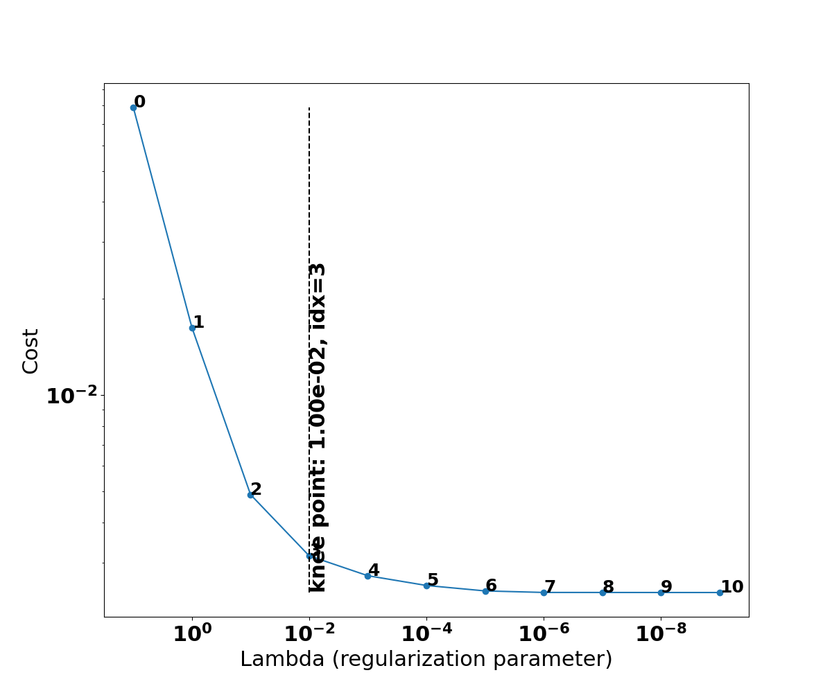
The estimator sweeps a range of deconvolution strengths and picks a "knee" on the L-curve of cost versus regularization — the point that balances noise suppression against over-fitting. Everything to the right of the knee mostly fits noise:

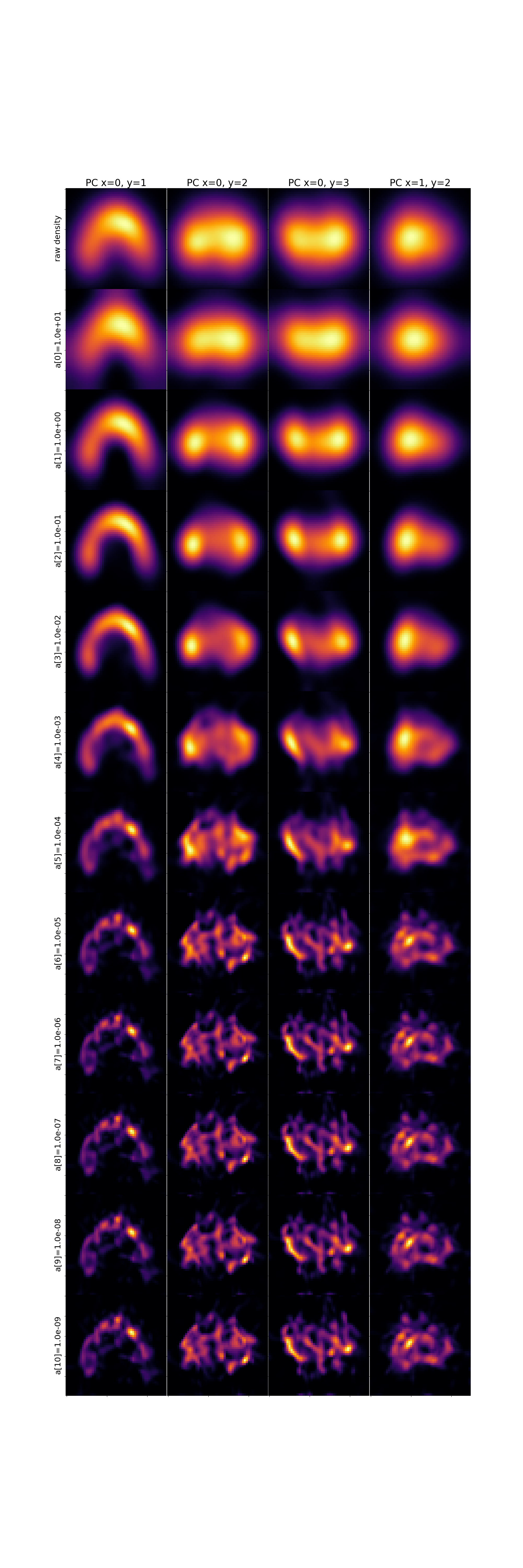
The deconvolved density at every regularization level is also saved as a grid, projected onto pairs of principal components. Heavily regularized estimates (top rows) are smooth and unimodal; lightly regularized ones (bottom rows) are sharper but noisier. The knee picks an intermediate level that reveals the distinct high-density basins — the stable conformational states — without over-fitting:

Estimating stable states

recovar estimate_stable_states density_output/data/deconv_density_knee.pkl \
    -o stable_states --n_local_maxs 1

Identifies local maxima of the conformational density — the most stable conformational states. The first argument is the density .pkl file produced by estimate_conformational_density; --n_local_maxs sets how many peaks to return (here, the single highest).

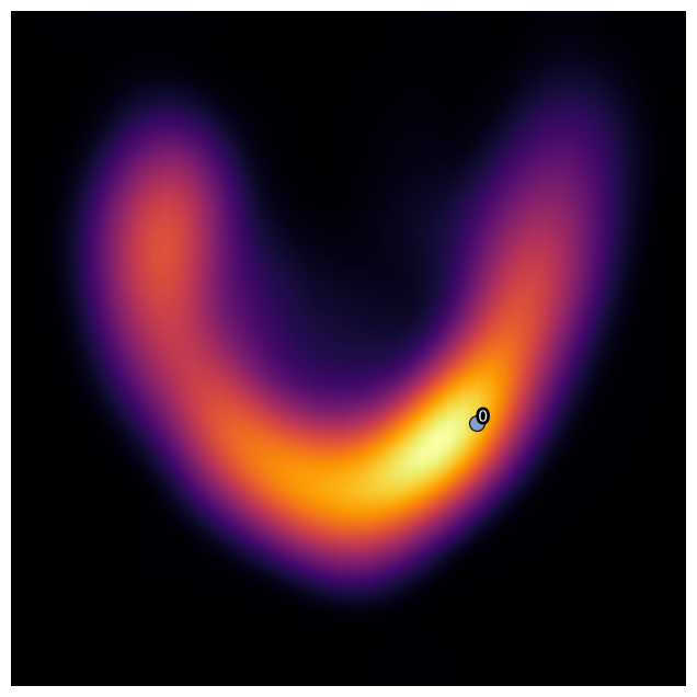
The marked point is the maximum of the density. It can look slightly off-peak here because the plot is only a 2D projection of the full 4-dimensional density — the true maximum sits where all four coordinates line up, not necessarily on the brightest spot of any single 2D view. Its coordinates are written to stable_state_0_coords.txt, ready to hand to compute_state to reconstruct that conformation.

Using density for trajectories

The density can guide trajectory computation to follow high-density paths:

recovar compute_trajectory output -o trajectory --zdim=4 \
    --density density_output/data/deconv_density_knee.pkl \
    --endpts centers.txt --ind 0,1

Pass the deconvolved density (deconv_density_knee.pkl) via --density so the path follows the sharp high-density regions. --zdim should match the density — the deconvolved density is computed in up to 4 dimensions, so --zdim=4 here.

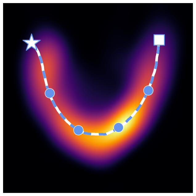
The dashed path runs from the start state (★) to the end state (■), bending to stay on the high-density ridge — threading through the populated basins rather than the empty region between them.

GUI alternative

In the GUI's latent space explorer, you can select two points on the scatter plot to compute a trajectory interactively. See the GUI Guide.

Using the GUI

In the web GUI (recovar gui), click New Job and select Density from the Job Type dropdown. Pick a completed pipeline job in the output picker, set the PCA Dimension, and (optionally) set Z Dimension Used under the Advanced section. Click Estimate Density to submit.

You can also reach density estimation from a completed pipeline job's Next Steps, which pre-fills the pipeline output for you.

After density estimation completes, use the Latent Space Explorer to color particles by conformational density and visually identify stable states.